Part 1: Delay quietly murders your bandwidth (spoiler: that 1/10 rule). Part 2: Architecture tricks to hide delay (cascaded loops, sensor fusion).
Part 3 is where we get cheeky: What if you could increase your PID gain by 39-158% while maintaining the same phase margin?
Sounds like snake oil? Let me show you the math. 🐍📊
The Problem: You're Leaving Gain on the Table
Remember from Part 1: delay forces you to cross unity gain early, wasting potential performance.
Your loop looks like this around crossover:
- Plant + PID: A nice first-order slope (think motor inertia, thermal lag)
- Delay: That jerk adding -ω·τ phase shift
You could crank up your PID gain... but then you'd blow past the -180° danger zone and turn your servo into a very expensive vibrator.
The insight: What if we could push the crossover frequency higher without losing phase margin?
Enter: The Lead Compensator (Your New Best Friend)
A lead compensator is deceptively simple:
$$ F(s) = \frac{1 + s/\omega_z}{1 + s/\omega_p}, \quad \omega_z < \omega_p $$
The magic is in what it does: - DC gain = 1 (your PID region stays completely untouched) - Adds positive phase between ωz and ωp (compensates for delay phase loss) - High-frequency gain = α where α = ωp/ωz (this is what we constrain)
Think of it as phase insurance: you're buying back some of the phase margin that delay stole, which lets you increase your DC gain.
The Real Objective (That Nobody Tells You)
Most tutorials say "maximize bandwidth." Yawn.
Here's what you actually care about: How much can I increase my PID gain?
Because higher gain means: - ✅ Better disturbance rejection - ✅ Tighter tracking - ✅ Lower steady-state error - ✅ More "stiffness" (the loop pushes back harder)
So instead of optimizing crossover frequency, we optimize the DC gain A directly.
The Model
Around crossover, your loop looks like:
$$ |L(j\omega)| = \frac{A}{\omega} $$
Where A is the gain we want to maximize. At the baseline crossover ω₁ (no lead):
$$ A_1 = \omega_{c1} = \frac{\pi/2 - \phi_m}{\tau} $$
With lead compensation, we can achieve A > A₁ while maintaining the same phase margin!
The Results (Prepare to Be Jealous)
Using COBYLA optimization with normalized variables (for tau-independence), here's what we get:
| Phase Margin | A₁ (baseline) | A (optimized) | Gain Improvement |
|---|---|---|---|
| 45° | 39.3 | 54.5 | +39% 🎉 |
| 60° | 26.2 | 43.8 | +67% 🚀 |
| 75° | 13.1 | 33.8 | +158% 🤯 |
Yeah, you read that right. 158% more gain at 75° phase margin.
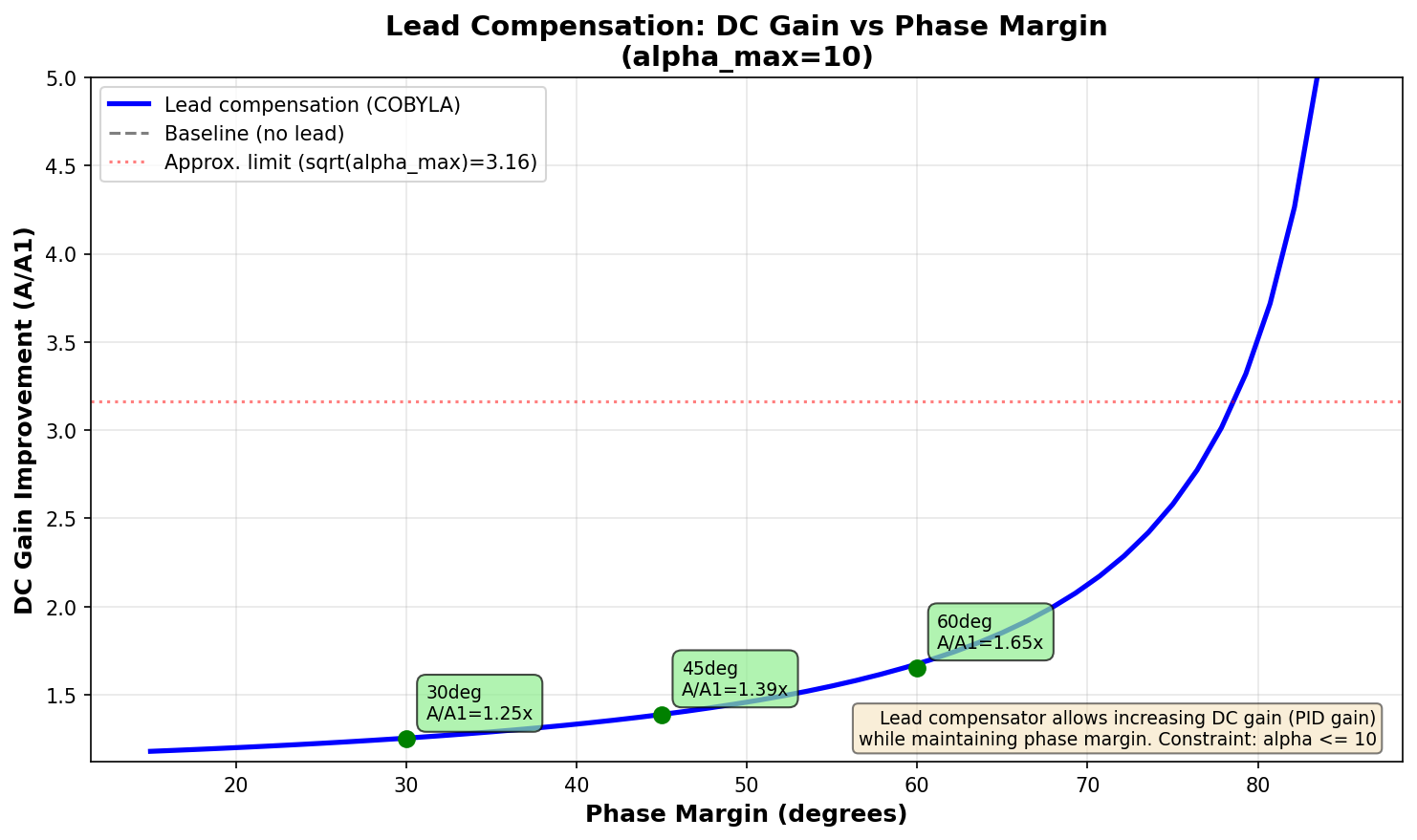
(Higher phase margin = more room to play = bigger improvements)
The Catch (Because There's Always a Catch)
The high-frequency gain α can't go to infinity because: - 📡 Sensor noise gets amplified (α acts like a gain knob for noise too) - 🎸 Unmodeled resonances wake up (your Bode plot doesn't know about that flex mode) - 🤖 Actuators get stressed (higher bandwidth = more demanding actuation)
Practical limit: α ≤ 10 (sometimes lower)
This is why we include it as a constraint in the optimizer, not a "nice to have."
Show Me the Math (For the Brave)
Full derivation with all the gory details: Lead Lag Math
Key equations: - Analytic crossover solution (quadratic in ω²) - Normalized optimization variables (A/A₁, ωz/ωc₁, α) - Phase margin constraint - Why the first-order slope model is valid
Spoiler: It's a 3D constrained optimization problem that would make your calculus professor proud.
Show Me the Code (For the Practical)
Python implementation: LeadCompensatorDesign
from lead_lag_design import LeadCompensatorDesign

# Design for 20ms delay, 45° phase margin
design = LeadCompensatorDesign(tau=0.02, phi_m_deg=45)

print(f"Baseline gain: A₁ = {design.A1:.2f}")
print(f"Optimized gain: A = {design.A:.2f}")
print(f"Improvement: {design.A/design.A1:.2f}x")
print(f"Lead zero: {design.wz:.2f} rad/s")
print(f"Lead pole: {design.wp:.2f} rad/s")
print(f"Alpha: {design.alpha:.2f}")
Output:
Baseline gain: A₁ = 39.27
Optimized gain: A = 54.49
Improvement: 1.39x  ← That's 39% more gain!
Lead zero: 43.31 rad/s
Lead pole: 433.13 rad/s
Alpha: 10.00
Features: - ✅ COBYLA optimizer with proper bounds - ✅ Normalized variables (tau-independent) - ✅ No silent failures (raises exceptions if infeasible) - ✅ Clean separation (import without matplotlib)
The Design Recipe
- Specify your requirements:
- Delay τ (include all delays: sample time, comms, filters)
- Phase margin φₘ (typically 45-60°)
-
Max α (default: 10, lower if you're noise-sensitive)
-
Run the optimizer:
- It maximizes DC gain A
- Enforces phase margin constraint
-
Keeps DC gain = 1 (PID region untouched)
-
Implement the lead:
- Zero at ωz
- Pole at ωp = α·ωz
-
Both well above your PID corner frequencies
-
Profit! (literally, if you're doing this for a living)
The Part Where I Admit the Dirty Secret
This all assumes your model is accurate around crossover. In practice: - That "first-order slope" might have a bump (unmodeled resonance) - Your delay estimate might be optimistic (firmware delays, anyone?) - Your sensor might be noisier than the datasheet suggested
Pro tip: Start with conservative α (5-6), not the maximum. Your future self will thank you during debugging at 2 AM.
Real Talk: When Does This Actually Work?
✅ Good candidates:
- Motor control (position/velocity loops)
- Thermal control (heaters, coolers)
- Pressure/flow control
- Any system with delay-limited bandwidth
❌ Bad candidates: - Systems with poorly known dynamics - Extremely noisy measurements - When you're already at the actuator limits
Takeaway
You don't need exotic hardware or black magic to improve control performance. Sometimes you just need: - Good models (that first-order slope around crossover) - Smart compensation (unity-gain lead) - Realistic constraints (cap that α!)
The lead compensator is like a performance optimizer for your control loop: it squeezes more gain out of the phase margin you already have.
Now the real question:
Have you ever added lead compensation and it worked perfectly in simulation... until real hardware reminded you about those unmodeled resonances? 😅
Drop your control horror stories below! 👇
The Series
- Control Loop Bandwidth - The 1/10 rule that ruins your day
- Improving Bandwidth - Architecture tricks (cascaded loops)
- Lead Compensation ← You are here
- Coming soon: Bode Phase Relationships & Lead-Lag Design
ControlSystems #PID #LeadCompensation #EmbeddedSystems #DSP #Robotics #MotionControl #RealTimeControl #Engineering
P.S. Yes, all the code and math are open source. Go break things responsibly. 🔧